
Trading is The Wrong Term for What Trading is - Research Article #72
How I calculate position size for continuous signals.

Hey there, Pedma here! Welcome to this ✨ free edition ✨ of the Trading Research Hub’s Newsletter. Each week, I'll share with you a blend of market research, personal trading experiences, and practical strategies, all aimed at making the world of systematic trading more relatable and accessible.
If you’re not a subscriber, here’s what you missed this past month so far:


If you’re not yet a part of our community, subscribe to stay updated with these more of these posts, and to access all our content.

You’re betting on a soccer match.
The bet is quite simple—if your team scores 3 goals by the end of the game, even if it loses, you win. Let’s add the optionality that you can bet at any point in the game, multiple times, and any amount you wish.
What’s the most important factor to decide the confidence in your bet? I’d say it is:
a) How many goals have been scored so far.
b) How much time do we have left.
I’ll be much more inclined to bet higher amounts at the 15 minute mark, on a 90 minute match, when my team has already scored 2 goals, than to bet at the 80 minute mark, when my team scored 0 goals, right?
So we’re saying that our confidence shifts as a function of the set of variables that mostly contribute to the outcome of our bet.
When scaling a position in a trade, why should it be any different? Why would we ignore the current set of variables the market realizes, and wait for arbitrary prices to execute our positions at?

That is what we will work on today. I want to answer the question of how do I scale a position, given the confidence on the current signal. Also this isn’t just theoretical, by the end of the article, our simple signal achieves a pretty impressive risk adjusted performance, despite the signal itself not being the focus today’s article.

Let’s get into it.
The Case for Continuous Signals
Many people criticize social media as a cesspool of noise. I tend to agree. But once in a blue moon, you find an absolute gem of a post as the one below by Agustin Lebron.

“Trading is the wrong term for what trading is. Trading is more accurately called positioning.”
Retail traders are often concerned about where to enter a trade or where to exit. This is not entirely wrong, but it is an inefficient way to view the market.
Fundamentally, when you trade, you buy stuff that you think it’s cheap, and sell stuff you think it’s expensive. You may be wondering, how does it apply to my SMA crossover signal or my moon cycles signal (half joking here). Well, it also applies, despite not being what’s promoted on traditional retail trader wisdom:
“You don’t predict markets, you react!"
That’s all nonsense.
Every time we enter a position, we’re implicitly making a prediction. The only question is how good of a prediction you make on average, and if it’s enough to pay for costs with some margin. That’s it. For example, let’s say that you have a breakout signal, and you want to play that as part of your trend-following signal. Maybe a 10-day breakout is a weaker signal than a 100-day breakout. One is more prone to noise than the other. So maybe we should scale more size as a function of the strength of the breakout, rather than a single arbitrary price level, that happened to work well historically.
We’ve briefly discussed this idea in our last article, where we scaled our position into multiple binary signals.
However, despite it not being wrong, it can be inefficient to only add/reduce size when we get new signals. This because a bunch of information is lost in the midst.
Let’s go back to our soccer match game, and ask a few questions:
What if the team has scored 1-goal, at the 25 minute mark, but we only take a bet after the 2-goal mark?
Is there no edge at all on betting on that 1-goal?
What if the only player that tends to score gets hurt and has to leave the game? Does that affect our bet?
What if the payoff of our bet decreases with the number of goals in the game?Maybe it behooves us to start taking positions early on in the game when the EV is at its highest.
Our optimal betting size is a moving function that should be adjusted based on what the game gives us, not on arbitrary rigid rules.
In the example plot below we can see a single allocation at the extremes of our signal. But what kind of information does a medium signal has? Why are we not exposed to it even if with just a fraction of a full position?

On a continuous spectrum, where positioning is evaluated periodically (each second, hour, day, etc), our exposure is much more dynamic and it adjusts to what we want it to be, based on our forecasts.

Obviously trading costs money and so you can’t just update your exposures every time it moves by a cent right? But you can much better capture the full scope of your edge by dynamically adjusting a position as it flows, if you really have edge.
Just like the soccer game where we bet based on our current confidence about the outcome of the game, we also can bet on the market as our confidence moves, and not only when we get an arbitrary signal.
So how do we calculate our continuous signal?
Overview of Signal Normalization
The first thing we need to do, is to define what kind of signal we’re going to use. This article will be more about how I currently do continuous signal scaling, rather than about the efficacy of a specific signal, so we’ll keep it simple.
The signal will be the distance of the close price of the asset we’re trading, to it’s 20-day simple moving average.
If we measure the % distance of the close price to the 20-sma, we can see that they highly differ from asset to asset. BTC for the past year has ranged from 25% to -15%, while XRP has ranged from -20% to 80%.
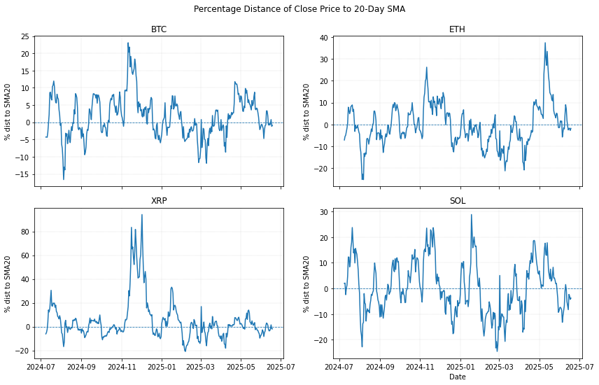
How would you then scale your positions to a maximum allocation? Would 40% be a 100% exposure? But then, the other assets never reached 40%, which means you were underexposed, even if the signal were at their extremes. Now consider if we add other less volatile assets such as equities, bonds, or commodities, what do we do then?
Well, we need to scale things so that we can compare apples to apples. We will use a simple volatility standardization, so that each signal is normalized to their volatility.
We’ll use the following formula to volatility scale our signal:
If you’re not much into math, don’t worry, it basically means this:
Price minus moving average – finds today’s gap from its 20-day average.
Divide by the moving average – turns that gap into a percentage-style measure.
Divide by the rolling 20-day volatility (σ) – scales the percentage by how much the price normally wiggles each day, giving a unit-free score that says how unusual the gap is relative to recent daily variability.
And these are the results we get when we plot our new values:
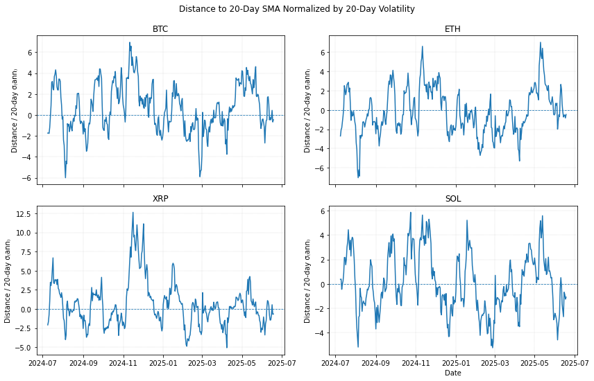
As you can see, they are much more evenly scaled when it comes to the maximum/minimum values, because now it’s scaled to their volatility. Even if the asset realizes 10% volatility or 100% volatility, it does not matter to the signal, all it matters is the relationship of the signal to it’s own asset’s idiosyncratic volatility.
Historic Range Scaling
(By the end of this section, I provide some code that I used to build this out.)
Now that we’re measuring apples to apples on all assets, we want to scale our position according to the signal.
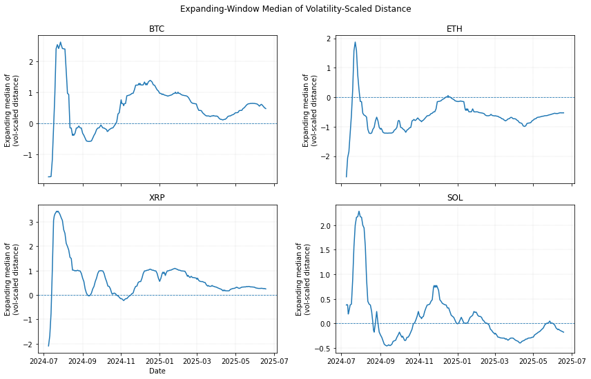
The first thing we want to do, is to take our normalized signal and calculate their expanding median. I will explain why we need this as we get deeper into the article. But basically we take all the values of the volatility scaled signal, and calculate the rolling median up until current time. When calculating the median, make sure it is up to current date (rolling), and not the entire available data, so that we do not induce hindsight bias into our tests!
Here’s the formula:
Simple explanation of the formula:
Collect every daily z-score so far – start at the very first valid observation and keep adding each new day’s Zt.
Take the median of that growing list – pick the middle value (the 50th-percentile).
Update the series each day – the result, Z̄t, shows the running “typical” deviation, smoothing out day-to-day noise while adapting as new data arrive.
Now, all we have to do is scale our signal. Why scale the signal? Think of the raw signal as a dial that tells you how much to invest. If the dial is usually small, you multiply it by a fixed number so that, on a normal day, the dial lands around +1 or –1. That “1” level is what you call “fully invested”.
s_t is the scaling factor at time t.
T is your target absolute size (
TARGET_ABS).m_t is the running median of absolute values up to time
In simple words we take the size we want (T) and divide it by how big values have typically been so far (the running median). If the typical size is small, the ratio is greater than 1 and stretches today’s value; if it’s large, the ratio is less than 1 and shrinks it.
Capping Extreme Values
In order to avoid excessive leverage when signals get too strong we need to set bounds to the scaled signal. Sometimes signals can get really strong, and we don’t want to infinitely allocate to a signal, no matter how strong that signal is. So we cap it between 2 and -2. Other systematic traders use other values, but that’s not relevant, it’s about what makes the most sense to you.
I prefer to cap it at 2/-2, because when we do position sizing, as we’ll see below, I can easily just use the intended size, and scale it to that 200% max position.
Don’t worry about the maths, I will provide the code below, and this is done in a single line of code.
Plain-English meaning:
Multiply today’s raw number by the scaling factor to stretch or shrink it.
If the result is bigger than C, set it to C; if it is smaller than −C, set it to −C.
Store the bounded result—nothing can exceed the safe band
This way, we are no longer getting values that would give us dangerous allocations.
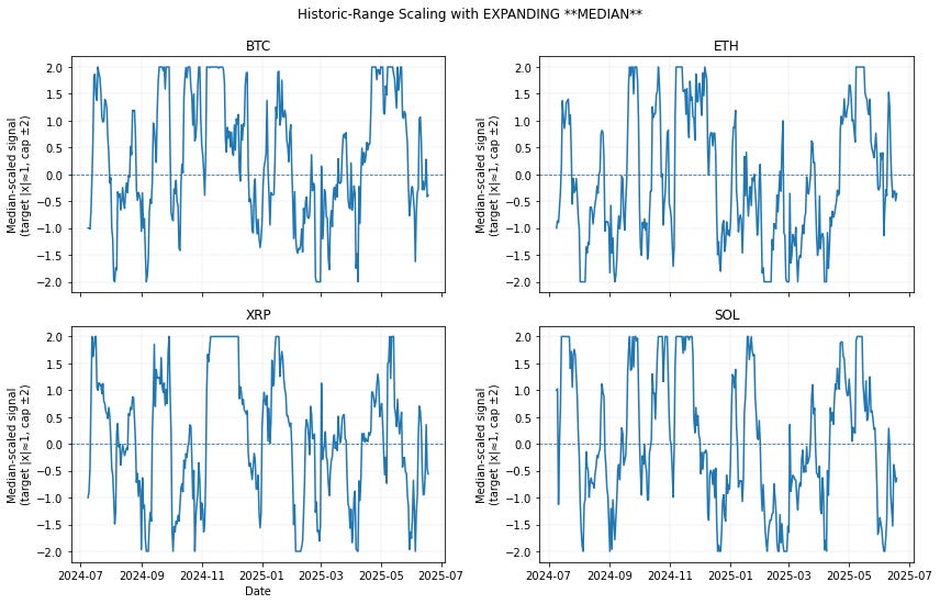
How does the Scaled Signal look like?
By using the median value to scale our signal, a handful of crazy spikes hardly move that middle value at all. Your scale stays based on what happens most of the time, not on once-in-a-blue-moon events. The dial now hits ±1 on ordinary days, so the strategy reaches full size just as intended.
Why not use only the raw signal and scale it?
The raw, volatility-adjusted signal (norm_dist) can range from tiny fractions to really high values. If you size positions directly off that unscaled number, two things happen:
Wild position swings – a quiet market gives you 1 unit of risk, a sudden pop gives you 15.
Unpredictable capital usage – you never know whether you’ll be 10 % or 400% invested tomorrow.
For example, let’s say that you use the maximum signal as your benchmark for a full allocation.

As you can see above, most of the time we don’t even get a full allocation, which means capital is always sitting on the sidelines, regardless of the potential of the signal. This is not efficient capital management. We need to be allocated when we have a decently strong signal.
This is why we use the median. Capital is optimally allocated given that historical median strong/weak signal.
I’ll also leave here some code for your own tests.
dfs = {}
for sym in SYMBOLS:
    df = get_klines(sym)

    # 20-day SMA and %-distance
    df["sma20"]     = df["close"].rolling(20).mean()
    df["dist_pct"]  = (df["close"] - df["sma20"]) / df["sma20"] * 100

    # 20-day daily volatility and z-score
    log_ret         = np.log(df["close"]).diff()
    df["vol20"]     = log_ret.rolling(20).std()
    df["norm_dist"] = df["dist_pct"] / (df["vol20"] * 100)

    # Expanding median of the z-score (already plotted in fig-3)
    df["exp_med"]   = df["norm_dist"].expanding().median()

    # ---------- NEW ➜ historic-range scalers ---------------------------------
    abs_series = df["norm_dist"].abs()

    # -- median-based scaler
    median_abs      = abs_series.expanding().median()
    scalar_median   = TARGET_ABS / median_abs.replace(0, np.nan)
    df["scaled_median"] = (df["norm_dist"] * scalar_median).clip(-CAP, CAP)

    dfs[sym] = df.dropna().reset_index(drop=True)
    sleep(0.15)   # gentle on Binance API
Incorporating Volatility Targeting for Stable Risk
Now that we have our signal, we need to size our positions, considering the most recent realized volatility of the individual asset we’re trading. I do this calculation right at the start of every position. For every position we want it to contribute the same amount of risk to our portfolio, regardless of how “jumpy” the market is that day. Here’s the formula I use:

This means that we get an allocation that is both scaled to the target annualized volatility we want to our portfolio and also the signal strength of the asset. Here’s some python code:
volatility_targeted_size = target_volatility / (max_signals_for_day * annualized_volatility_20) * total_equity

volatility_targeted_size *= scaled_median_signal
Let’s now look at those equity curves!
Trading System Parameters
Before we move on to our data, let’s first define the rules of the trading models we will be testing.
Base Metrics
Signal Timeframe: Daily
Maximum Leverage: 2x
Maximum Number of Open Positions: 20
Position Direction: Long/Short
Signal Type: Continuous
Ranking: Asset’s 20-day dollar volume (highest to lowest)
Compounding: Enabled
Fees + Slippage (per order): 6 bps
Target Volatility: 40%
Iteration 1
Long Signals:
Position is scaled as a relationship to the 20-SMA. (see Overview of Signal Normalization section)
Short Signals:
Position is scaled as a relationship to the 20-SMA. (see Overview of Signal Normalization section)
Position size is calculated as a function of the scaled position and volatility of the asset.
Performance Overview
As we’ve discussed earlier in this article, the signal is not important today. We’ve used a pretty simplistic signal, but ideally we’d want as many signals as possible, obviously within the same group of what we’re trying to get exposure to, to make sure we have a long-term robust model. Despite its simplicity, we were able to produce some impressive risk adjusted returns when compared to the benchmarks, which is the whole point of this exercise.
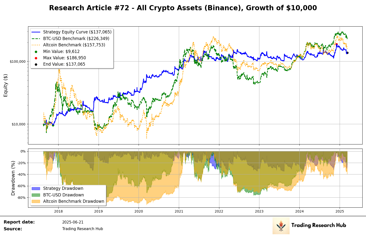

The drawdown went from a 93% for the crypto market benchmark, and 83% for BTC buy and hold, to a 34% for our strategy. The average drawdown went from 55% and 42% to about 15% on our strategy. This is highly significant when going through the wild ride of the market.
The next natural step will be to look for better signals, and put them into a blend, so that we can capture multiple regimes and also not be exposed to a single indicator.
I hope you’ve enjoyed today’s article!
Ps… Looking to Work With Me?
After testing 100’s of trading strategies and spending 1,000’s of hours studying trading and building my own models, I had a few clients reach out to work with me and the outcomes have been quite good so far!
I’ve helped multiple clients now:
Develop their first systematic model
Help reviewing their current trading processes
Build solid frameworks on trading system development
Stop wasting money and time on bad ideas
Develop better risk management models
And much more…
If you want my custom help on your trading business, or would like to work with me, book a free 15-minute consultation call:
And finally, I’d love your input on how I can make Trading Research Hub even more useful for you!
Disclaimer: The content and information provided by the Trading Research Hub, including all other materials, are for educational and informational purposes only and should not be considered financial advice or a recommendation to buy or sell any type of security or investment. Always conduct your own research and consult with a licensed financial professional before making any investment decisions. Trading and investing can involve significant risk of loss, and you should understand these risks before making any financial decisions.
Nice article! One question I have, where does TARGET_ABS come from? What does that represent?